背景与目的
Rossmann (劳诗曼)要求预测位于德国的 1,115 家商店2015年8,9月份的 6
周日销售额。可靠的销售预测使商店经理能够制定有效的员工时间表,从而提高工作效率和积极性。
(如果文章中的公式不能正常显示,请刷新该页面。如果还不能解决,请邮箱联系我,谢谢...)
Rossmann 在 7 个欧洲国家经营着 3,000 多家日化用品超市。目前,
Rossmann
商店经理的任务是提前最多六周预测他们的每日销售额。商店销售受许多因素影响,包括促销、竞争、学校和州假期、季节性和地点。由于成千上万的经理根据他们的独特情况预测销售,因此结果的准确性可能参差不齐。
这就是算法和零售、物流邻域的一次深度融合,从而提前备货,减少库存,提升资金周转率,促进公司更加健康发展,为员工更合理的工作、休息提供合理安排,为工作效率的提高保驾护航
数据介绍
一共1115 家 Rossmann 商店的历史销售数据。任务是预测测试集的 “Sales”
列。请注意,数据集中的一些商店已暂时关闭以进行翻新
大多数字段都是字面含义,以下是一些字段的说明
字段 说明
Store
每个商店唯一的ID
Sales
销售额
Customers
销售客户数
Open
商店是否营业 0=关闭,1=开业
StateHoliday
国家假日
SchoolHoliday
学校假日
StoreType
店铺类型:a,b,c,d
Assortment
产品组合级别:a=基本,b=附加,c=扩展
CompetitionDistance
距离最近的竞争对手距离(米)
CompetitionOpenSince[Month/Year]
最近的竞争对手开业时间
Promo
指店铺当日是否在进行促销
Promo2
指店铺是否在进行连续促销
0=未进行,1=正在进行
Promo2Since[Year/Week]
商店开始参与Promo2的时间
PromoInterval
促销期
StateHoliday:通常所有店铺都在国家假日关门:a=公共假日,b=复活节假日,c=圣诞节,0=无
数据加载
查看数据
导库
1
2
3
4
5
6
7
8
import pandas as pdimport numpy as npimport matplotlib.pyplot as pltimport seaborn as snsimport xgboost as xgbimport warningswarnings.filterwarnings('ignore' ) import time
读取数据
1
2
3
4
5
train = pd.read_csv('./data/rossmann-store-sales/train.csv' , dtype={'StateHoliday' :np.string_}) test = pd.read_csv('./data/rossmann-store-sales/test.csv' , dtype={'StateHoliday' :np.string_}) store = pd.read_csv('./data/rossmann-store-sales/store.csv' )
展示数据
1 display(train.head(), test.head(), store.head())
1
2
3
4
5
6
7
8
9
10
11
12
13
14
15
16
17
18
19
20
21
22
23
24
25
26
27
28
29
30
31
32
33
34
35
36
37
38
39
40
41
42
43
44
# 输出 -----------------------------train---------------------------- Store DayOfWeek Date Sales Customers Open Promo StateHoliday \ 0 1 5 2015-07-31 5263 555 1 1 0 1 2 5 2015-07-31 6064 625 1 1 0 2 3 5 2015-07-31 8314 821 1 1 0 3 4 5 2015-07-31 13995 1498 1 1 0 4 5 5 2015-07-31 4822 559 1 1 0 SchoolHoliday 0 1 1 1 2 1 3 1 4 1 -------------------------------test---------------------------------- Id Store DayOfWeek Date Open Promo StateHoliday SchoolHoliday 0 1 1 4 2015-09-17 1.0 1 0 0 1 2 3 4 2015-09-17 1.0 1 0 0 2 3 7 4 2015-09-17 1.0 1 0 0 3 4 8 4 2015-09-17 1.0 1 0 0 4 5 9 4 2015-09-17 1.0 1 0 0 --------------------------------store---------------------------- Store StoreType Assortment CompetitionDistance CompetitionOpenSinceMonth \ 0 1 c a 1270.0 9.0 1 2 a a 570.0 11.0 2 3 a a 14130.0 12.0 3 4 c c 620.0 9.0 4 5 a a 29910.0 4.0 CompetitionOpenSinceYear Promo2 Promo2SinceWeek Promo2SinceYear \ 0 2008.0 0 NaN NaN 1 2007.0 1 13.0 2010.0 2 2006.0 1 14.0 2011.0 3 2009.0 0 NaN NaN 4 2015.0 0 NaN NaN PromoInterval 0 NaN 1 Jan,Apr,Jul,Oct 2 Jan,Apr,Jul,Oct 3 NaN 4 NaN
查看数据规模
1 print (train.shape, test.shape, store.shape)
1
2
# 输出 (1017209, 9) (41088, 8) (1115, 10)
发现数据集还是很庞大,训练集有百万条数据
数据清洗
空数据处理
1 display(train.info(), test.info(), store.info())
1
2
3
4
5
6
7
8
9
10
11
12
13
14
15
16
17
18
19
20
21
22
23
24
25
26
27
28
29
30
31
32
33
34
35
36
37
38
39
40
41
42
43
44
45
46
47
48
49
# 输出 <class 'pandas.core.frame.DataFrame'> RangeIndex: 1017209 entries, 0 to 1017208 Data columns (total 9 columns): # Column Non-Null Count Dtype --- ------ -------------- ----- 0 Store 1017209 non-null int64 1 DayOfWeek 1017209 non-null int64 2 Date 1017209 non-null object 3 Sales 1017209 non-null int64 4 Customers 1017209 non-null int64 5 Open 1017209 non-null int64 6 Promo 1017209 non-null int64 7 StateHoliday 1017209 non-null object 8 SchoolHoliday 1017209 non-null int64 dtypes: int64(7), object(2) memory usage: 69.8+ MB <class 'pandas.core.frame.DataFrame'> RangeIndex: 41088 entries, 0 to 41087 Data columns (total 8 columns): # Column Non-Null Count Dtype --- ------ -------------- ----- 0 Id 41088 non-null int64 1 Store 41088 non-null int64 2 DayOfWeek 41088 non-null int64 3 Date 41088 non-null object 4 Open 41077 non-null float64 5 Promo 41088 non-null int64 6 StateHoliday 41088 non-null object 7 SchoolHoliday 41088 non-null int64 dtypes: float64(1), int64(5), object(2) memory usage: 2.5+ MB <class 'pandas.core.frame.DataFrame'> RangeIndex: 1115 entries, 0 to 1114 Data columns (total 10 columns): # Column Non-Null Count Dtype --- ------ -------------- ----- 0 Store 1115 non-null int64 1 StoreType 1115 non-null object 2 Assortment 1115 non-null object 3 CompetitionDistance 1112 non-null float64 4 CompetitionOpenSinceMonth 761 non-null float64 5 CompetitionOpenSinceYear 761 non-null float64 6 Promo2 1115 non-null int64 7 Promo2SinceWeek 571 non-null float64 8 Promo2SinceYear 571 non-null float64 9 PromoInterval 571 non-null object dtypes: float64(5), int64(2), object(3) memory usage: 87.2+ KB
我们发现只有测试集和商店集存在缺失数据
处理测试集空数据
由于测试集仅仅缺失11个数据,我们查看所有缺失的数据
1 test[test['Open' ].isnull()]
1
2
3
4
5
6
7
8
9
10
11
12
13
14
15
16
17
18
19
20
21
22
23
24
25
26
# 输出 Id Store DayOfWeek Date Open Promo StateHoliday \ 479 480 622 4 2015-09-17 NaN 1 0 1335 1336 622 3 2015-09-16 NaN 1 0 2191 2192 622 2 2015-09-15 NaN 1 0 3047 3048 622 1 2015-09-14 NaN 1 0 4759 4760 622 6 2015-09-12 NaN 0 0 5615 5616 622 5 2015-09-11 NaN 0 0 6471 6472 622 4 2015-09-10 NaN 0 0 7327 7328 622 3 2015-09-09 NaN 0 0 8183 8184 622 2 2015-09-08 NaN 0 0 9039 9040 622 1 2015-09-07 NaN 0 0 10751 10752 622 6 2015-09-05 NaN 0 0 SchoolHoliday 479 0 1335 0 2191 0 3047 0 4759 0 5615 0 6471 0 7327 0 8183 0 9039 0 10751 0
我们发现缺失数据全部都是622号商店
我们查看622商店历史开店比例,看看该商店是不是活跃店铺
1
2
3
4
sum_open = train[train['Store' ]==622 ]['Open' ].sum () sum_day = train[train['Store' ]==622 ]['Open' ].count() open_percent = sum_open/sum_day print (f'开店比例为:{open_percent:.2 f} ' )
622商店开店率为83%而另外17%可以断定为节假日观点,所以判断622商店为活跃店铺
将缺失的11条数据的缺失字段 Open 填充为1
1 2 3 test.fillna(1 , inplace=True ) test.info()
处理商店空数据
查看缺失数据
1 2 3 4 5 6 7 8 9 10 11 12 # 输出 Store 0 StoreType 0 Assortment 0 CompetitionDistance 3 CompetitionOpenSinceMonth 354 CompetitionOpenSinceYear 354 Promo2 0 Promo2SinceWeek 544 Promo2SinceYear 544 PromoInterval 544 dtype: int64
发现缺失数据中,有两组缺失数据的缺失数量相同,而 CompetitionDistance
字段仅仅缺失三个数据
1 2 3 4 5 6 7 8 9 v1 = 'CompetitionDistance' v2 = 'CompetitionOpenSinceMonth' v3 = 'CompetitionOpenSinceYear' v4 = 'Promo2SinceWeek' v5 = 'Promo2SinceYear' v6 = 'PromoInterval'
其中两组缺失数据相同,猜测存在同时缺失
1 2 store[(store[v2].isnull()) & (store[v3].isnull())].shape
1 store[(store[v4].isnull()) & (store[v5].isnull()) & (store[v6].isnull())].shape
印证了我们的说法,这两组数据确实是同时缺失
缺失的这些数据分布表示竞争对手相关字段和促销相关字段,我们可以解释为新店开业暂时没有竞争对手以及促销活动,将这些数据全部填充为0
1 2 store.fillna(0 , inplace=True ) store.info()
1 2 3 4 5 6 7 8 9 10 11 12 13 14 15 16 17 18 # 输出 <class 'pandas.core.frame.DataFrame'> RangeIndex: 1115 entries, 0 to 1114 Data columns (total 10 columns): # Column Non-Null Count Dtype --- ------ -------------- ----- 0 Store 1115 non-null int64 1 StoreType 1115 non-null object 2 Assortment 1115 non-null object 3 CompetitionDistance 1115 non-null float64 4 CompetitionOpenSinceMonth 1115 non-null float64 5 CompetitionOpenSinceYear 1115 non-null float64 6 Promo2 1115 non-null int64 7 Promo2SinceWeek 1115 non-null float64 8 Promo2SinceYear 1115 non-null float64 9 PromoInterval 1115 non-null object dtypes: float64(5), int64(2), object(3) memory usage: 87.2+ KB
空数据处理完毕
销售数据同时间的关系
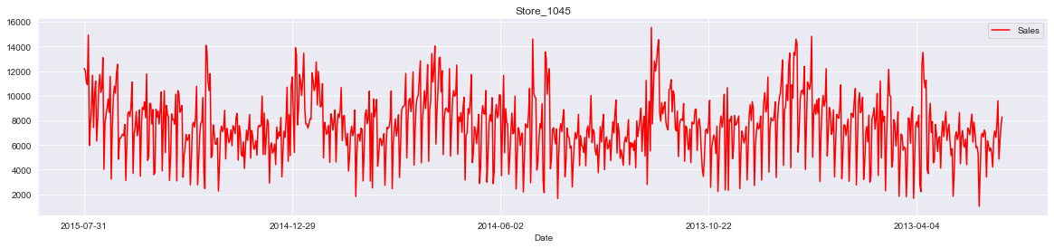
1 2 3 sales_date = train[train['Sales' ]>0 ] store_id = 1045 sales_date[sales_date['Store' ] == store_id].plot(x='Date' , y='Sales' , figsize=(20 , 4 ), color='red' , title=f'Store_{store_id} ' )
从图中可以看出店铺的销售额是有周期性变化的,一年中11,12月份销量相对较高,可能是季节(圣诞节)因素或者促销等原因
此外从2014年6-9月的销量来看,6,7月份的销售趋势与8,9月份类似,而我们需要预测的6周在2015年8,9月份,因此我们可以把2015年6,7月份最近6周的1115家店的数据作为测试数据,用于模型的优化和验证
特征工程
数据合并
将训练数据和测试数据同商店数据进行合并,顺便舍去那些销售额小于0的异常数据
1 2 3 4 5 train = train[train['Sales' ]>0 ] train = pd.merge(train, store, on='Store' , how='left' ) test = pd.merge(test, store, on='Store' , how='left' ) display(train.shape, test.shape)
1 2 3 # 输出 (844338, 18) (41088, 17)
合并过滤后,训练数据从百万变成了80万,可见销售额小于0的数据很多
非数字类型数据转换
时间数据处理
时间数据为object,需要转为数字形式;同时促销日期为月份形式,将其与实际月份进行映射,构建
IsPromo 字段确定该月是否促销
1 2 3 4 5 6 7 8 9 10 11 12 13 14 for data in [train, test]: data['Year' ] = data['Date' ].apply(lambda x: x.split('-' )[0 ]).astype(int ) data['Month' ] = data['Date' ].apply(lambda x: x.split('-' )[1 ]).astype(int ) data['Day' ] = data['Date' ].apply(lambda x: x.split('-' )[2 ]).astype(int ) Month2str = {1 :'Jan' , 2 :'Feb' , 3 :'Mar' , 4 :'Apr' , 5 :'May' , 6 :'Jun' , 7 :'Jul' , 8 :'Aug' , 9 :'Sep' , 10 :'Oct' , 11 :'Nov' , 12 :'Dec' } data['MonthStr' ] = data['Month' ].map (Month2str) data['IsPromo' ] = data.apply(lambda x: 0 if x['PromoInterval' ]==0 else 1 if x['MonthStr' ] in x['PromoInterval' ] else 0 , axis=1 )
其他非数字类型处理
StateHoliday、StoreType、Assortment
字段中含有字母,将其转为数字类型
1 2 3 4 5 6 for data in [train, test]: mappings = {'0' :0 , 'a' :1 , 'b' :2 , 'c' :3 , 'd' :4 } data['StateHoliday' ] = data['StateHoliday' ].map (mappings) data['StoreType' ] = data['StoreType' ].map (mappings) data['Assortment' ] = data['Assortment' ].map (mappings)
将上述二者代码合并:
1 2 3 4 5 6 7 8 9 10 11 12 13 14 15 16 17 for data in [train, test]: data['Year' ] = data['Date' ].apply(lambda x: x.split('-' )[0 ]).astype(int ) data['Month' ] = data['Date' ].apply(lambda x: x.split('-' )[1 ]).astype(int ) data['Day' ] = data['Date' ].apply(lambda x: x.split('-' )[2 ]).astype(int ) Month2str = {1 :'Jan' , 2 :'Feb' , 3 :'Mar' , 4 :'Apr' , 5 :'May' , 6 :'Jun' , 7 :'Jul' , 8 :'Aug' , 9 :'Sep' , 10 :'Oct' , 11 :'Nov' , 12 :'Dec' } data['MonthStr' ] = data['Month' ].map (Month2str) data['IsPromo' ] = data.apply(lambda x: 0 if x['PromoInterval' ]==0 else 1 if x['MonthStr' ] in x['PromoInterval' ] else 0 , axis=1 ) mappings = {'0' :0 , 'a' :1 , 'b' :2 , 'c' :3 , 'd' :4 } data['StateHoliday' ] = data['StateHoliday' ].map (mappings) data['StoreType' ] = data['StoreType' ].map (mappings) data['Assortment' ] = data['Assortment' ].map (mappings)
构建训练数据和测试数据
根据下面的结构分别构建数据
删除无关特征
通过之前的特征工程,产生了一系列新特征,将这些特征的母特征删除,以及一些对后续处理无用的特征删除
1 2 3 4 5 df_train = train.drop(['Date' , 'PromoInterval' , 'MonthStr' , 'Customers' , 'Open' ], axis=1 ) df_test = test.drop(['Date' , 'PromoInterval' , 'MonthStr' , 'Open' , 'Id' ], axis=1 ) display(df_train.shape, df_test.shape)
数据切片
1 2 3 4 5 X_test = df_train[:6 *7 *1115 ] X_train = df_train[6 *7 *1115 :] display(X_train.shape, X_test.shape)
1 2 3 # 输出 (797508, 18) (46830, 18)
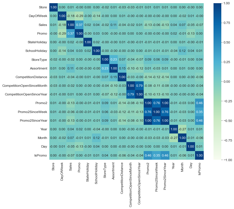
绘制相关性系数
1 2 3 plt.figure(figsize=(12 , 10 )) plt.rcParams['font.size' ] = 12 sns.heatmap(df_train.corr(), annot=True , cmap='GnBu' , fmt='.2f' , vmin=-1 , vmax=1 )
提取模型训练数据
目标值正态化
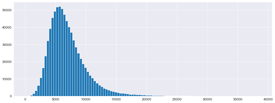
查看目标值 Sales 的分布
1 2 plt.figure(figsize=(16 , 6 )) _ = plt.hist(X_train['Sales' ], bins=100 )
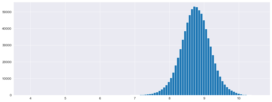
正态分布偏左,需要将其“摆正”,使用对数化即可完成操作
1 2 3 4 5 6 7 8 y_train = np.log1p(X_train['Sales' ]) y_test = np.log1p(X_test['Sales' ]) X_train = X_train.drop(['Sales' ], axis=1 ) X_test = X_test.drop(['Sales' ], axis=1 ) plt.figure(figsize=(16 , 6 )) _ = plt.hist(y_train, bins=100 )
构建模型
定义评价函数
使用RMSPE(均方根百分比误差)评价函数:分数越低模型越好 \[
RMSPE=\sqrt{\frac{1}{N}\sum^{N}_{i=1}(1-\frac{\hat{y}}{y})^2}
\]
1 2 3 4 5 6 7 8 9 10 11 12 13 14 15 def rmspe (y, yhat ): return np.sqrt(np.mean((1 -yhat/y)**2 )) def rmspe_xp (y, yhat ): y = np.expm1(y) yhat = np.expm1(yhat.get_label()) return 'rmspe_xp' , np.sqrt(np.mean((1 -yhat/y)**2 )) ''' return name, data - name: 返回评估函数名称,替换原评估函数名称 - data:返回评估分数 '''
模型训练
使用 XGBoost 模型以及网格搜索进行超参数优化
1 2 3 4 5 6 7 8 9 10 11 12 13 14 15 16 17 18 19 20 21 22 23 24 25 %%time params = {'objective' : 'reg:linear' , 'booster' :'gbtree' , 'eta' : 0.03 , 'max_depth' : 10 , 'subsample' : 0.9 , 'colsample_bytree' : 0.7 , 'silent' :1 , 'seed' :10 } num_boost_round = 6000 dtrain = xgb.DMatrix(X_train, y_train) dtest = xgb.DMatrix(X_test, y_test) evals = [(dtrain, 'train' ), (dtest, 'validation' )] ''' evals = [训练, 验证] - 训练:(data, name) - 验证:(data, name) data:对应的数据 name:为对应数据命名,替换原数据名称 ''' gbm = xgb.train(params, dtrain, num_boost_round, evals=evals, early_stopping_rounds=100 , feval=rmspe_xp, verbose_eval=10 )
params参数说明
objective:定义需要被最小化的优化函数
reg:linear:线性回归(默认)
reg:logistic:逻辑回归
binary:logistic:二分类的逻辑回归,返回概率
multi:softmax:使用softmax多分类器,返回预测类别
booster:树类型
eta:与GBM中的learning_rate类似,减少每一步的权重,提高鲁棒性(默认0.3)
max_depth:最大数深度
subsample:为每个树创建训练集时使用所有数据的比例(采样比例)
colsample_bytree:每个分裂节点使用全部特征的比例
silent:输出信息(1=关闭)
seed:随机种子
xgb.train()参数
params:字典,传入模型参数
dtrain:训练数据
num_boost_round:训练轮次(决策树数量)
evals:验证,评估的数据
early_stopping_rounds:早停法参数,在N次训练没有提升后结束训练
feval:模型评价函数
verbose_eval:
True:打印输出日志,每次训练详情
数字:每隔N个输出一次日志
xgb_model:训练之前用于加载的xgb_model
保存模型
1 2 gbm.save_model('.../trained_model.json' )
模型评估
使用RMSPE_XP评分
1 2 3 4 5 6 7 8 X_test.sort_index(inplace=True ) y_test.sort_index(inplace=True ) yhat = gbm.predict(xgb.DMatrix(X_test)) error = rmspe(np.expm1(y_test), np.expm1(yhat)) print (f'RMSPE_XP: {error} ' )
1 2 # 输出 RMSPE_XP: 0.1286831991891701
将模型评估结构作为新数据加到原数据中
1 2 3 4 5 6 7 8 9 10 res = pd.DataFrame(data=y_test) res['Prediction' ] = yhat res = pd.merge(X_test, res, left_index=True , right_index=True ) res['Ratio' ] = res['Prediction' ] / res['Sales' ] res['Error' ] = abs (1 - res['Ratio' ]) res['Weight' ] = res['Sales' ] / res['Prediction' ]
可视化
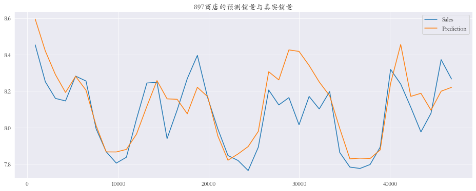
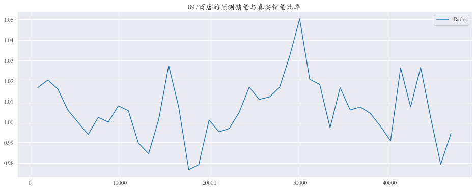
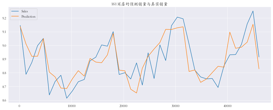
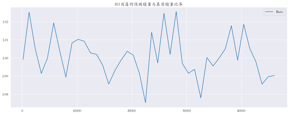
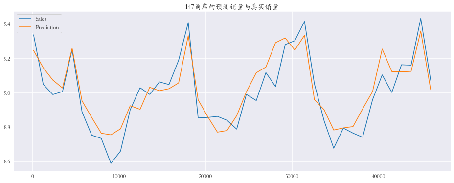
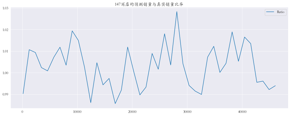
随机抽取三个商店进行可视化
1 2 3 4 5 6 7 8 9 10 11 12 13 14 15 plt.rcParams['font.family' ] = 'STKaiti' col_1 = ['Sales' , 'Prediction' ] col_2 = ['Ratio' ] shops = np.random.randint(1 , 1116 , size=3 ) print ('所有商店的预测值和真实销量的比率%.3f' % res['Ratio' ].mean())print ('所有商店的预测值和真实销量的比率%.3f' % res['Ratio' ].mean())for shop in shops: data_col_1 = res[res['Store' ] == shop][col_1] data_col_2 = res[res['Store' ] == shop][col_2] data_col_1.plot(title=f'{shop} 商店的预测销量与真实销量' , figsize=(16 , 6 )) data_col_2.plot(title=f'{shop} 商店的预测销量与真实销量比率' , figsize=(16 , 6 ))
对数据进行矫正
全局矫正
查看偏差数据
1 2 res.sort_values(by='Error' , ascending=False )
1 2 3 4 5 6 7 8 9 10 11 12 # 查看误差最大的前10条数据 Error 0.234481 0.182347 0.180231 0.138051 0.137430 0.120414 0.115215 0.114456 0.111926 0.111843
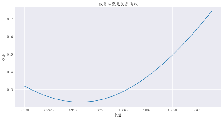
对预测值进行微调 :对预测值乘上权重参数
1 2 3 4 5 6 7 8 9 10 11 12 13 14 15 weights = [(0.99 + (i/1000 )) for i in range (20 )] errors = [] for w in weights: error = rmspe(np.expm1(y_test), np.expm1(yhat * w)) errors.append(error) errors = pd.Series(errors, index=weights) index = errors.argmin() print (f'最小误差权重为: {weights[index]} , 最小误差为: {errors.iloc[index]} ' )print (index)errors.plot(title='权重与误差关系曲线' , figsize=(12 , 6 )) plt.xlabel('权重' ) plt.ylabel('误差' )
查看权重从0.990到1.010的误差,选择最小值
1 2 # 输出 最小误差权重为: 0.996, 最小误差为: 0.122778807130969026
对每个商店进行矫正
1 2 3 4 5 6 7 8 9 10 11 12 13 14 15 16 17 18 19 20 21 22 23 24 25 26 27 28 29 30 31 32 33 34 35 36 37 shops = range (1 , 1116 ) weights1 = [] weights2 = [] for shop in shops: df1 = res[res['Store' ] == shop][col_1] df2 = df_test[df_test['Store' ] == shop] weights = [(0.98 + (i/1000 )) for i in range (40 )] errors = [] for w in weights: error = rmspe(np.expm1(df1['Sales' ]), np.expm1(df1['Prediction' ] * w)) errors.append(error) errors = pd.Series(errors, index=weights) index = errors.argmin() best_weight = np.array(weights[index]) weights1.extend(best_weight.repeat(len (df1)).tolist()) weights2.extend(best_weight.repeat(len (df2)).tolist()) X_test = X_test.sort_values(by='Store' ) X_test['Weights1' ] = weights1 X_test = X_test.sort_index() weights1 = X_test['Weights1' ] X_test = X_test.drop(['Weights1' ], axis=1 ) df_test = df_test.sort_values(by='Store' ) df_test['Weights2' ] = weights2 df_test = df_test.sort_index() weights2 = df_test['Weights2' ] df_test = df_test.drop(['Weights2' ], axis=1 ) yhat_new = yhat * weights1 print (f'最小误差: {rmspe(np.expm1(y_test), np.expm1(yhat_new))} ) len(df_test)
1 2 # 输出 最小误差: 0.11452434988887741
模型预测
1 2 3 4 5 6 7 y_pred = gbm.predict(xgb.DMatrix(df_test)) result = pd.DataFrame({'ID' :range (1 , len (df_test) + 1 ), 'Sales' :np.expm1(y_pred * weights2)}) result.to_csv('./data/rossmann-store-sales/result.csv' , index=False )
提交
总结
通过 Rossmann
商店销售预测模型,一个算法和零售、物流邻域深度融合的项目,加深了对这类模型的应用技巧,提高机器学习应用能力
同时也学习了一些思路,机器学习模型在预测时有一些倾向:对于这类回归模型来说,可能偏大也可能偏小,我们可以根据预测结果对结果进行微调,以平衡模型的这种倾向
如有任何问题可以留言或者点击左侧邮箱联系...