项目介绍
项目需解决的问题
通过利用信用卡历史交易数据记录,构建信用卡反欺诈预测模型,提前发现客户信用卡被盗刷的行为
建模思路
构建信用卡反欺诈预测模型:
场景解析(算法选择)
数据预处理
特征工程
特征衍生
特征选择
特征缩放
模型训练
模型评估与优化
项目背景
数据集包含由欧洲持卡人于2013年9月使用信用卡进行交易的数据,此数据集显示两天内发生的交易,其中284807笔交易中有492笔被盗刷。数据集非常不平衡,Positive类(被盗刷)占所有交易的0.172%
数据只包含作为PCA转换结果的数字输入变量。不幸的是,由于保密问题,我们无法提供有关数据的原始功能和更多背景信息。特征V1,V2,...V28是使用PCA获得的主要特征,没有使用PCA转换的唯一特征是
”时间“ 和 “金额” 。特征 “时间”
包含数据集中每个事务和第一个事务之间经过的秒数。特征 “金额”
是交易金额,此特征可用于实际依赖的成本认知学习。特征 “类别”
是响应变量,如果发生盗刷,则为1,否则为0
场景解析
算法选择
该项目的目标是找到盗刷的交易记录,即一笔交易分为正常与不正常,为二分类问题,且数据都已含有标签,是一个监督学习场景,我们可以选择逻辑回归算法(Logistic
Regression)
数据分析
数据已经是结构化数据,不需要做特征抽象(针对有序和无序的文本分类型特征,采用不同的方法进行处理,将其类别属性数值化)。特征V1至V28是经过PCA处理,而特征Time和Amount的数据规格与其他特征差别较大,需要对其做特征缩放,将特征缩放至同一规格。在数据质量方面,没有出现乱码或空字符的数据,可以确定字段Class为目标列,其他列为特征列
模型评估
数据是已经标注的数据,可以使用交叉验证对训练集生成的模型进行评估,80%的数据进行训练,20%的数据进行预测和评估
场景总结
对于该业务场景总结:
根据历史记录数据学习并对信用卡持卡人是否会发生盗刷行为进行预测,二分类监督学习场景,选择逻辑回归算法(Logistic
Regression)
数据为结构化数据,不需要做特征抽象,但需要做特征缩放
数据预处理
导包并加载数据
1 2 3 4 5 6 7 8 9 10 11 12 13 14 15 16 17 18 19 20 import warningswarnings.filterwarnings('ignore' ) import pandas as pdpd.set_option('display.float_format' , lambda x: '%.2f' % x) import numpy as npimport matplotlib.pyplot as pltimport matplotlib.gridspec as gridspecimport seaborn as snsimport missingno as msno from sklearn.linear_model import LogisticRegressionfrom sklearn.ensemble import RandomForestClassifierfrom sklearn.model_selection import train_test_splitfrom sklearn.model_selection import GridSearchCVfrom sklearn.metrics import roc_auc_score, auc, roc_curve, recall_score, accuracy_score, classification_reportfrom sklearn.preprocessing import StandardScaler
1 2 data = pd.read_csv('.../creditcard.csv' )
查看前5条数据
1
2
3
4
5
6
7
8
9
10
11
12
13
14
15
16
# 输出 Time V1 V2 V3 V4 V5 V6 V7 V8 V9 ... V21 V22 \ 0 0.00 -1.36 -0.07 2.54 1.38 -0.34 0.46 0.24 0.10 0.36 ... -0.02 0.28 1 0.00 1.19 0.27 0.17 0.45 0.06 -0.08 -0.08 0.09 -0.26 ... -0.23 -0.64 2 1.00 -1.36 -1.34 1.77 0.38 -0.50 1.80 0.79 0.25 -1.51 ... 0.25 0.77 3 1.00 -0.97 -0.19 1.79 -0.86 -0.01 1.25 0.24 0.38 -1.39 ... -0.11 0.01 4 2.00 -1.16 0.88 1.55 0.40 -0.41 0.10 0.59 -0.27 0.82 ... -0.01 0.80 V23 V24 V25 V26 V27 V28 Amount Class 0 -0.11 0.07 0.13 -0.19 0.13 -0.02 149.62 0 1 0.10 -0.34 0.17 0.13 -0.01 0.01 2.69 0 2 0.91 -0.69 -0.33 -0.14 -0.06 -0.06 378.66 0 3 -0.19 -1.18 0.65 -0.22 0.06 0.06 123.50 0 4 -0.14 0.14 -0.21 0.50 0.22 0.22 69.99 0 [5 rows x 31 columns]
查看后5条数据
1
2
3
4
5
6
7
8
9
10
11
12
13
14
15
16
# 输出 Time V1 V2 V3 V4 V5 V6 V7 V8 V9 ... \ 284802 172786.00 -11.88 10.07 -9.83 -2.07 -5.36 -2.61 -4.92 7.31 1.91 ... 284803 172787.00 -0.73 -0.06 2.04 -0.74 0.87 1.06 0.02 0.29 0.58 ... 284804 172788.00 1.92 -0.30 -3.25 -0.56 2.63 3.03 -0.30 0.71 0.43 ... 284805 172788.00 -0.24 0.53 0.70 0.69 -0.38 0.62 -0.69 0.68 0.39 ... 284806 172792.00 -0.53 -0.19 0.70 -0.51 -0.01 -0.65 1.58 -0.41 0.49 ... V21 V22 V23 V24 V25 V26 V27 V28 Amount Class 284802 0.21 0.11 1.01 -0.51 1.44 0.25 0.94 0.82 0.77 0 284803 0.21 0.92 0.01 -1.02 -0.61 -0.40 0.07 -0.05 24.79 0 284804 0.23 0.58 -0.04 0.64 0.27 -0.09 0.00 -0.03 67.88 0 284805 0.27 0.80 -0.16 0.12 -0.57 0.55 0.11 0.10 10.00 0 284806 0.26 0.64 0.38 0.01 -0.47 -0.82 -0.00 0.01 217.00 0 [5 rows x 31 columns]
时间单位以秒为单位
查看数据信息
1
2
3
4
5
6
7
8
9
10
11
12
13
14
15
16
17
18
19
20
21
22
23
24
25
26
27
28
29
30
31
32
33
34
35
36
37
38
39
# 输出 <class 'pandas.core.frame.DataFrame'> RangeIndex: 284807 entries, 0 to 284806 Data columns (total 31 columns): # Column Non-Null Count Dtype --- ------ -------------- ----- 0 Time 284807 non-null float64 1 V1 284807 non-null float64 2 V2 284807 non-null float64 3 V3 284807 non-null float64 4 V4 284807 non-null float64 5 V5 284807 non-null float64 6 V6 284807 non-null float64 7 V7 284807 non-null float64 8 V8 284807 non-null float64 9 V9 284807 non-null float64 10 V10 284807 non-null float64 11 V11 284807 non-null float64 12 V12 284807 non-null float64 13 V13 284807 non-null float64 14 V14 284807 non-null float64 15 V15 284807 non-null float64 16 V16 284807 non-null float64 17 V17 284807 non-null float64 18 V18 284807 non-null float64 19 V19 284807 non-null float64 20 V20 284807 non-null float64 21 V21 284807 non-null float64 22 V22 284807 non-null float64 23 V23 284807 non-null float64 24 V24 284807 non-null float64 25 V25 284807 non-null float64 26 V26 284807 non-null float64 27 V27 284807 non-null float64 28 V28 284807 non-null float64 29 Amount 284807 non-null float64 30 Class 284807 non-null int64 dtypes: float64(30), int64(1) memory usage: 67.4 MB
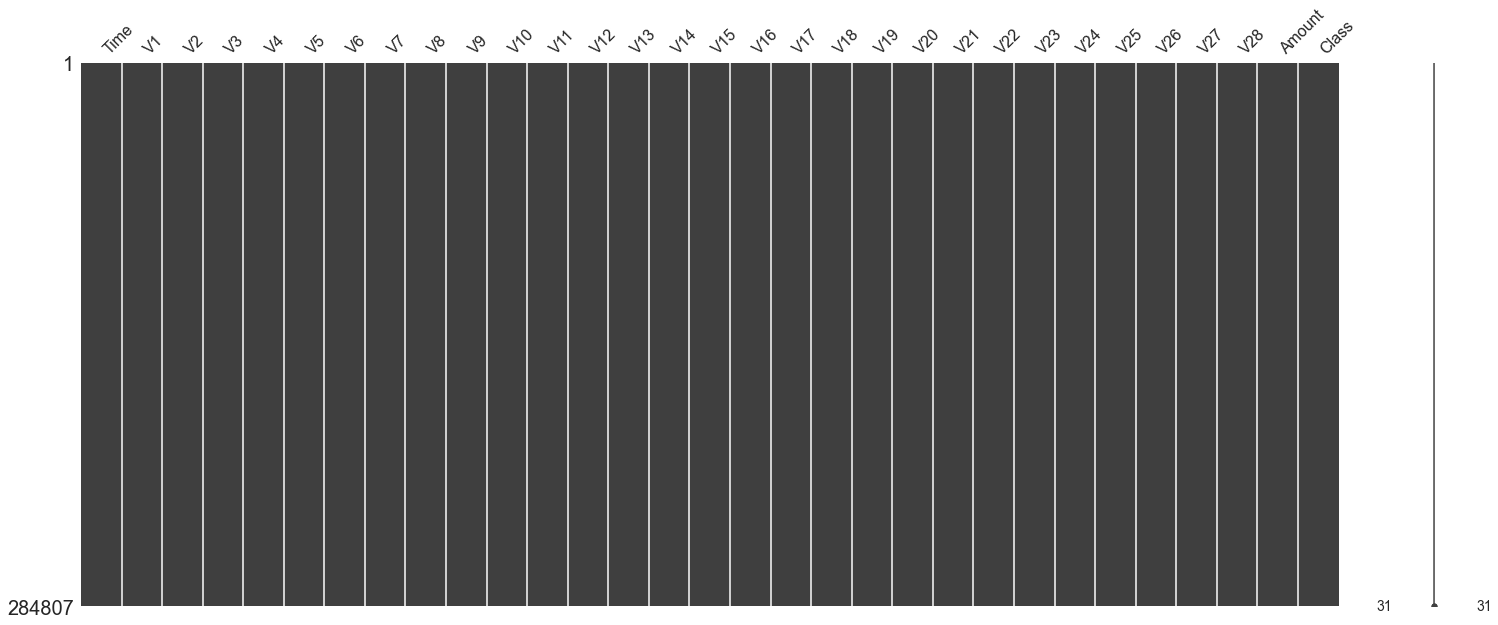
查看空数据
数据干净无缺失数据
查看数据的统计学特征
1 2 3 4 5 6 7 8 9 10 11 12 13 14 15 16 17 18 19 20 21 22 23 24 25 26 27 28 29 30 31 32 33 34 35 36 37 38 39 40 41 42 43 44 45 46 47 48 49 50 51 52 53 54 55 56 57 58 59 60 61 62 63 64 65 66 # 输出 count mean std min 25% 50% 75% \ Time 284807.00 94813.86 47488.15 0.00 54201.50 84692.00 139320.50 V1 284807.00 0.00 1.96 -56.41 -0.92 0.02 1.32 V2 284807.00 0.00 1.65 -72.72 -0.60 0.07 0.80 V3 284807.00 -0.00 1.52 -48.33 -0.89 0.18 1.03 V4 284807.00 0.00 1.42 -5.68 -0.85 -0.02 0.74 V5 284807.00 0.00 1.38 -113.74 -0.69 -0.05 0.61 V6 284807.00 0.00 1.33 -26.16 -0.77 -0.27 0.40 V7 284807.00 -0.00 1.24 -43.56 -0.55 0.04 0.57 V8 284807.00 0.00 1.19 -73.22 -0.21 0.02 0.33 V9 284807.00 -0.00 1.10 -13.43 -0.64 -0.05 0.60 V10 284807.00 0.00 1.09 -24.59 -0.54 -0.09 0.45 V11 284807.00 0.00 1.02 -4.80 -0.76 -0.03 0.74 V12 284807.00 -0.00 1.00 -18.68 -0.41 0.14 0.62 V13 284807.00 0.00 1.00 -5.79 -0.65 -0.01 0.66 V14 284807.00 0.00 0.96 -19.21 -0.43 0.05 0.49 V15 284807.00 0.00 0.92 -4.50 -0.58 0.05 0.65 V16 284807.00 0.00 0.88 -14.13 -0.47 0.07 0.52 V17 284807.00 -0.00 0.85 -25.16 -0.48 -0.07 0.40 V18 284807.00 0.00 0.84 -9.50 -0.50 -0.00 0.50 V19 284807.00 0.00 0.81 -7.21 -0.46 0.00 0.46 V20 284807.00 0.00 0.77 -54.50 -0.21 -0.06 0.13 V21 284807.00 0.00 0.73 -34.83 -0.23 -0.03 0.19 V22 284807.00 -0.00 0.73 -10.93 -0.54 0.01 0.53 V23 284807.00 0.00 0.62 -44.81 -0.16 -0.01 0.15 V24 284807.00 0.00 0.61 -2.84 -0.35 0.04 0.44 V25 284807.00 0.00 0.52 -10.30 -0.32 0.02 0.35 V26 284807.00 0.00 0.48 -2.60 -0.33 -0.05 0.24 V27 284807.00 -0.00 0.40 -22.57 -0.07 0.00 0.09 V28 284807.00 -0.00 0.33 -15.43 -0.05 0.01 0.08 Amount 284807.00 88.35 250.12 0.00 5.60 22.00 77.16 Class 284807.00 0.00 0.04 0.00 0.00 0.00 0.00 max Time 172792.00 V1 2.45 V2 22.06 V3 9.38 V4 16.88 V5 34.80 V6 73.30 V7 120.59 V8 20.01 V9 15.59 V10 23.75 V11 12.02 V12 7.85 V13 7.13 V14 10.53 V15 8.88 V16 17.32 V17 9.25 V18 5.04 V19 5.59 V20 39.42 V21 27.20 V22 10.50 V23 22.53 V24 4.58 V25 7.52 V26 3.52 V27 31.61 V28 33.85 Amount 25691.16 Class 1.00
我们发现特征V1~V28都已经归一化,而Amount数据与其他特征差距过大
特征工程
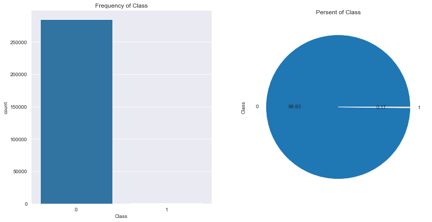
目标变量探索
1
2
3
4
5
6
7
8
fig, axes = plt.subplots(1 , 2 , figsize=(14 ,7 )) sns.countplot(x='Class' , data=data, ax=axes[0 ]) axes[0 ].set_title('Frequency of Class' ) data['Class' ].value_counts().plot(kind='pie' , autopct='%1.2f' , ax=axes[1 ]) axes[1 ].set_title('Persent of Class' )
样本严重不均衡
特征衍生
时间跨度太大,以秒为单位,将其转为小时
1 data['Hour' ] = data['Time' ].apply(lambda x: divmod (x, 3600 )[0 ])
特征选择
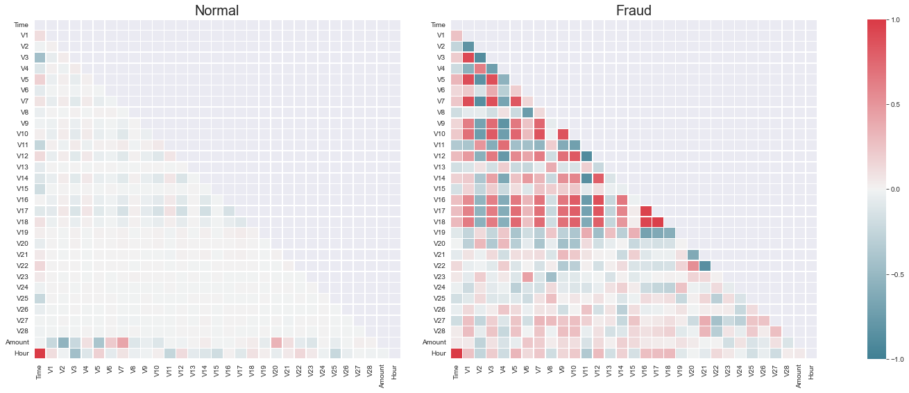
正常与不正常数据的区别
1 2 3 4 5 6 7 8 9 10 11 12 13 14 15 16 17 18 19 20 21 22 23 24 Xfraud = data.loc[data['Class' ] == 1 ] Xnonfraud = data.loc[data['Class' ] == 0 ] correlationNonFraud = Xnonfraud.loc[:,Xnonfraud.columns != 'Class' ].corr() mask = np.zeros_like(correlationNonFraud) indices = np.triu_indices_from(mask) mask[indices] = True kw = {'width_ratios' : (1 , 1 , 0.05 ), 'wspace' : 0.2 } f, (ax1, ax2, cbar_ax) = plt.subplots(1 , 3 , figsize=(22 , 9 ), gridspec_kw=kw) cmap = sns.diverging_palette(220 , 10 , as_cmap=True ) ax1 = sns.heatmap(correlationNonFraud, ax = ax1, vmin=-1 , vmax=1 , cmap=cmap, square=False , linewidths=0.5 , mask=mask, cbar=False ) ax1.set_title('Normal' , size=20 ) correlationFraud = Xfraud.loc[:,Xfraud.columns != 'Class' ].corr() cmap = sns.diverging_palette(220 , 10 , as_cmap=True ) ax2 = sns.heatmap(correlationFraud, ax = ax2, vmin=-1 , vmax=1 , cmap=cmap, square=False , linewidths=0.5 , mask=mask, cbar_ax=cbar_ax, cbar_kws={'orientation' : 'vertical' , 'ticks' : [-1 , -0.5 , 0 , 0.5 , 1 ]}) ax2.set_title('Fraud' , size=20 )
从图中看出,正常交易的数据和异常交易的数据的特征有明显区别,异常交易数据与某些特征有很强的关系,可以利用这些特征将正常交易与异常交易进行区分
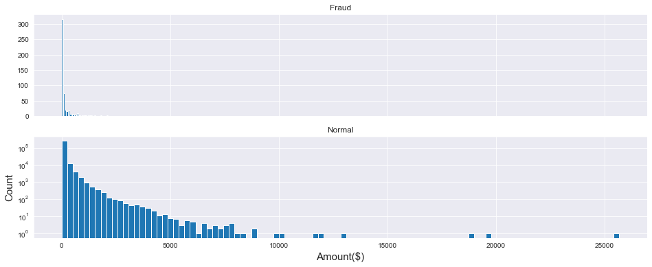
交易额与交易次数的关系
1
2
3
4
5
6
7
8
9
10
f, (ax1, ax2) = plt.subplots(2 , 1 , sharex=True , figsize=(16 , 6 )) plt.yscale('log' ) plt.xlabel('Amount($)' ,size=15 ) plt.ylabel('Count' ,size=15 ) ax1.hist(data['Amount' ][data['Class' ] == 1 ], bins=30 ) ax1.set_title('Fraud' ) ax2.hist(data['Amount' ][data['Class' ] == 0 ], bins=100 ) ax2.set_title('Normal' )
从图中看出,盗刷者更倾向于小金额,以避免被卡主发现
交易时间和交易次数的关系
1 sns.catplot(x='Hour' , data=data, kind='count' , palette='autumn' , size=6 , aspect=3 )
从图中可以发现,每天早上9点到晚上11点是消费高峰期
交易金额与交易时间的关系
1
2
3
4
5
6
7
8
9
f, (ax1, ax2) = plt.subplots(2 , 1 , sharex=True , figsize=(16 , 6 )) plt.xlabel('Hour(H)' ,size=15 ) plt.ylabel('Count' ,size=15 ) ax1.scatter(x=data['Hour' ][data['Class' ] == 1 ], y=data['Amount' ][data['Class' ] == 1 ]) ax1.set_title('Fraud' ) ax2.scatter(x=data['Hour' ][data['Class' ] == 0 ], y=data['Amount' ][data['Class' ] == 0 ]) ax2.set_title('Normal' )
从图中也可以看出,正常的交易金额区间是很大的,大部分都在5000以下,而盗刷的金额在500以下,盗刷者更倾向小金额
盗刷者盗刷时间关系
1 sns.catplot(x='Hour' , data=data[data['Class' ]==1 ], kind='count' , palette='autumn' , size=6 , aspect=3 )
从图中看出,在盗刷样本中,离群值出现在消费低谷期,也就是晚上11点到第二天早上9点,说明盗刷者喜欢在卡主睡觉时作案,防止引起卡主注意
不同特征下盗刷与正常数据的分布
1
2
3
4
5
6
7
8
9
10
11
12
v_feat = data.iloc[:,1 :29 ].columns plt.rcParams['font.family' ] = 'STKaiTi' plt.figure(figsize=(16 , 4 *28 )) gs = gridspec.GridSpec(28 , 1 ) for i, v in enumerate (v_feat): ax = plt.subplot(gs[i]) sns.distplot(data[v][data['Class' ]==1 ], bins=50 ) sns.distplot(data[v][data['Class' ]==0 ], bins=100 ) ax.set_title(f'{v} 的特征分布' , size=15 )
我们的任务是将正常消费与盗刷进行区分,在这些特征中,找出那些盗刷与正常消费能够区分的特征作为最终特征,把那些区分度不高的特征进行舍去
将特征
V8、V13、V15、V20、V21、V22、V23、V24、V25、V26、V27、V28舍去,留下其余特征
1
2
3
4
drop_list = ['V8' ,'V13' ,'V15' ,'V20' ,'V21' ,'V22' ,'V23' ,'V24' ,'V25' ,'V26' ,'V27' ,'V28' ,'Time' ] new_data = data.drop(drop_list, axis=1 ) new_data.shape new_data.head()
1
2
3
4
5
6
7
8
9
10
11
12
13
14
# 输出 V1 V2 V3 V4 V5 V6 V7 V9 V10 V11 V12 V14 \ 0 -1.36 -0.07 2.54 1.38 -0.34 0.46 0.24 0.36 0.09 -0.55 -0.62 -0.31 1 1.19 0.27 0.17 0.45 0.06 -0.08 -0.08 -0.26 -0.17 1.61 1.07 -0.14 2 -1.36 -1.34 1.77 0.38 -0.50 1.80 0.79 -1.51 0.21 0.62 0.07 -0.17 3 -0.97 -0.19 1.79 -0.86 -0.01 1.25 0.24 -1.39 -0.05 -0.23 0.18 -0.29 4 -1.16 0.88 1.55 0.40 -0.41 0.10 0.59 0.82 0.75 -0.82 0.54 -1.12 V16 V17 V18 V19 Amount Class Hour 0 -0.47 0.21 0.03 0.40 149.62 0 0.00 1 0.46 -0.11 -0.18 -0.15 2.69 0 0.00 2 -2.89 1.11 -0.12 -2.26 378.66 0 0.00 3 -1.06 -0.68 1.97 -1.23 123.50 0 0.00 4 -0.45 -0.24 -0.04 0.80 69.99 0 0.00
特征标准化
由于时间和金额的特征的数值差异过大,需要进行标准化,有利于梯度下降
1
2
3
4
5
col = ['Amount' ,'Hour' ] sc = StandardScaler() new_data[col] = sc.fit_transform(new_data[col]) new_data.head()
1
2
3
4
5
6
7
8
9
10
11
12
13
14
# 输出 V1 V2 V3 V4 V5 V6 V7 V9 V10 V11 V12 V14 \ 0 -1.36 -0.07 2.54 1.38 -0.34 0.46 0.24 0.36 0.09 -0.55 -0.62 -0.31 1 1.19 0.27 0.17 0.45 0.06 -0.08 -0.08 -0.26 -0.17 1.61 1.07 -0.14 2 -1.36 -1.34 1.77 0.38 -0.50 1.80 0.79 -1.51 0.21 0.62 0.07 -0.17 3 -0.97 -0.19 1.79 -0.86 -0.01 1.25 0.24 -1.39 -0.05 -0.23 0.18 -0.29 4 -1.16 0.88 1.55 0.40 -0.41 0.10 0.59 0.82 0.75 -0.82 0.54 -1.12 V16 V17 V18 V19 Amount Class Hour 0 -0.47 0.21 0.03 0.40 0.24 0 -1.96 1 0.46 -0.11 -0.18 -0.15 -0.34 0 -1.96 2 -2.89 1.11 -0.12 -2.26 1.16 0 -1.96 3 -1.06 -0.68 1.97 -1.23 0.14 0 -1.96 4 -0.45 -0.24 -0.04 0.80 -0.07 0 -1.96
查看标准化后的统计学特征
1
2
3
4
5
6
7
8
9
10
11
12
13
14
15
16
17
18
19
20
21
# 输出 count mean std min 25% 50% 75% max V1 284807.00 0.00 1.96 -56.41 -0.92 0.02 1.32 2.45 V2 284807.00 0.00 1.65 -72.72 -0.60 0.07 0.80 22.06 V3 284807.00 -0.00 1.52 -48.33 -0.89 0.18 1.03 9.38 V4 284807.00 0.00 1.42 -5.68 -0.85 -0.02 0.74 16.88 V5 284807.00 0.00 1.38 -113.74 -0.69 -0.05 0.61 34.80 V6 284807.00 0.00 1.33 -26.16 -0.77 -0.27 0.40 73.30 V7 284807.00 -0.00 1.24 -43.56 -0.55 0.04 0.57 120.59 V9 284807.00 -0.00 1.10 -13.43 -0.64 -0.05 0.60 15.59 V10 284807.00 0.00 1.09 -24.59 -0.54 -0.09 0.45 23.75 V11 284807.00 0.00 1.02 -4.80 -0.76 -0.03 0.74 12.02 V12 284807.00 -0.00 1.00 -18.68 -0.41 0.14 0.62 7.85 V14 284807.00 0.00 0.96 -19.21 -0.43 0.05 0.49 10.53 V16 284807.00 0.00 0.88 -14.13 -0.47 0.07 0.52 17.32 V17 284807.00 -0.00 0.85 -25.16 -0.48 -0.07 0.40 9.25 V18 284807.00 0.00 0.84 -9.50 -0.50 -0.00 0.50 5.04 V19 284807.00 0.00 0.81 -7.21 -0.46 0.00 0.46 5.59 Amount 284807.00 0.00 1.00 -0.35 -0.33 -0.27 -0.04 102.36 Class 284807.00 0.00 0.04 0.00 0.00 0.00 0.00 1.00 Hour 284807.00 -0.00 1.00 -1.96 -0.82 -0.22 0.92 1.60
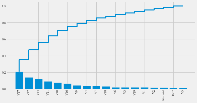
特征重要性
查看各个特征的贡献,利用随机森林的feature_importances_对其进行重要性排序
1 2 3 4 5 6 7 8 9 10 11 12 13 14 15 16 17 18 19 20 21 22 23 24 25 26 27 28 features = list (new_data.columns) features.remove('Class' ) X = new_data[features] Y = new_data['Class' ] from sklearn.ensemble import RandomForestClassifierclf = RandomForestClassifier() clf.fit(X, Y) importances = clf.feature_importances_ plt.rcParams['figure.figsize' ] = (12 , 6 ) plt.style.use('fivethirtyeight' ) feat_name = features index = np.argsort(importances)[::-1 ] importances = importances[index] feat_name = np.array(feat_name) feat_name = feat_name[index] plt.xticks(range (18 ), feat_name, rotation=90 , fontsize=14 ) plt.bar(range (18 ), importances) plt.step(range (18 ), np.cumsum(importances))
模型训练
过采样
之前提到,数据的目标列Class呈现较大的样本不平衡,会对模型的学习造成困扰,解决样本不平衡常用的解决方法有过采样(扩充样本较少的部分)和欠采样(减少样本较多的部分)本项目使用的是过采样方法,具体使用的是SMOTE(Synthetic
Minority Oversampling Technique)
1 2 3 4 5 6 7 8 9 10 11 from imblearn.over_sampling import SMOTEX = new_data[features] y = new_data['Class' ] y.value_counts() smote = SMOTE() X, y = smote.fit_resample(X, y) y.value_counts()
1
2
3
4
# 输出 1 284315 0 284315 Name: Class, dtype: int64
训练样本已经达到平衡
算法建模与混淆矩阵
使用逻辑回归建模
1
2
3
4
model = LogisticRegression() model.fit(X, y) y_ = model.predict(X) print (accuracy_score(y, y_))
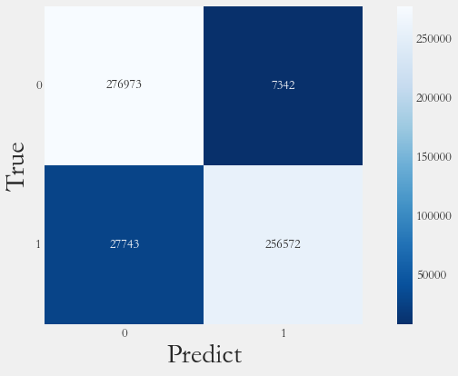
混淆矩阵
1 2 3 4 from sklearn.metrics import confusion_matrixcm = confusion_matrix(y, y_) print (cm)
1 2 3 # 输出 [[276973 7342] [ 27743 256572]]
召回率
1 2 3 recall = cm[1 ,1 ] / (cm[1 ,1 ] + cm[1 ,0 ]) print (recall)
可视化
1 2 3 4 ax = sns.heatmap(data=cm, square=True , cmap='Blues_r' , annot=cm, fmt='d' ) plt.xlabel('Predict' ,fontsize=30 ) plt.ylabel('True' ,fontsize=30 ) ax.set_yticklabels(labels=ax.get_yticklabels(), rotation=0 )
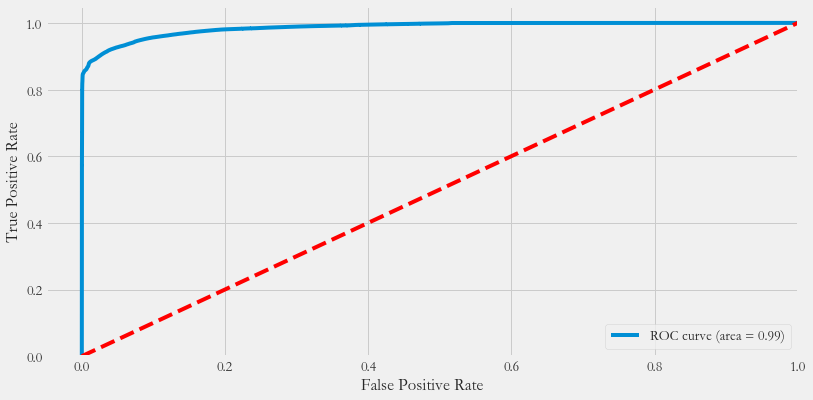
ROC、AUC
1 2 3 4 5 6 7 8 9 10 11 12 13 y_pre = model.predict_proba(X)[:,1 ] fpr, tpr, thresholds = roc_curve(y, y_pre) roc_auc = auc(fpr, tpr) plt.plot(fpr, tpr, label='ROC curve (area = %0.2f)' % roc_auc) plt.legend(loc="lower right" ) plt.plot([0 , 1 ], [0 , 1 ], 'k--' , color='r' ) plt.xlim([-0.05 , 1.0 ]) plt.ylim([0.0 , 1.05 ]) plt.xlabel('False Positive Rate' ) plt.ylabel('True Positive Rate' )
交叉验证
1 2 3 4 5 6 x_train, x_test, y_train, y_test = train_test_split(X, y, test_size=0.2 ) param_grid = {'C' : [0.01 , 0.1 , 1 , 10 , 100 , 1000 ], 'penalty' : ['l1' , 'l2' ]} gs = GridSearchCV(LogisticRegression(), param_grid, cv=10 ) gs.fit(x_train, y_train)
查看网格搜索结果
1 2 3 4 results = pd.DataFrame(gs.cv_results_) print ('Best Parameters: ' , gs.best_params_)print ('Best score: ' , gs.best_score_)
1 2 3 # 输出 Best Parameters: {'C': 0.1, 'penalty': 'l2'} Best score: 0.9384265657808122
准确率评估
1 2 y_predict = gs.predict(x_test) print ('Accuracy: ' , accuracy_score(y_test, y_predict))
1 2 # 输出 Accuracy: 0.9371383852417213
1 2 from sklearn.metrics import classification_reportprint (classification_report(y_test, y_predict))
1 2 3 4 5 6 7 8 9 # 输出 precision recall f1-score support 0 0.91 0.97 0.94 56836 1 0.97 0.90 0.93 56890 accuracy 0.94 113726 macro avg 0.94 0.94 0.94 113726 weighted avg 0.94 0.94 0.94 113726
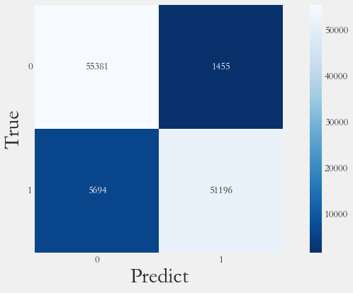
混淆矩阵
1 2 3 4 5 6 cm_pred = confusion_matrix(y_test, y_predict) ax = sns.heatmap(data=cm_pred, square=True , cmap='Blues_r' , annot=cm_pred, fmt='d' ) plt.xlabel('Predict' ,fontsize=30 ) plt.ylabel('True' ,fontsize=30 ) ax.set_yticklabels(labels=ax.get_yticklabels(), rotation=0 )
阈值调整
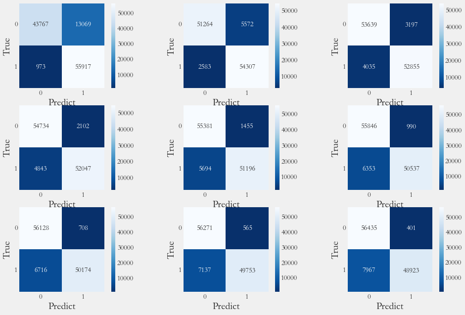
不同阈值的混淆矩阵
1 2 3 4 5 6 7 8 9 10 11 12 13 14 15 16 17 18 19 20 21 22 y_pre_proba = gs.predict_proba(x_test)[:,1 ] thresholds = [0.1 , 0.2 , 0.3 , 0.4 , 0.5 , 0.6 , 0.7 , 0.8 , 0.9 ] plt.figure(figsize=(15 , 10 )) np.set_printoptions(precision=2 ) j = 1 for t in thresholds: y_pre = y_pre_proba >= t plt.subplot(3 , 3 , j) j += 1 cnf_matrix = confusion_matrix(y_test, y_pre) print ('召回率为: ' , cnf_matrix[1 , 1 ]/(cnf_matrix[1 , 0 ] + cnf_matrix[1 , 1 ]), end='\t' ) print ('准确率为: ' , (cnf_matrix[0 , 0 ] + cnf_matrix[1 , 1 ]) / cnf_matrix.sum ()) ax = sns.heatmap(data=cnf_matrix, square=True , cmap='Blues_r' , annot=cnf_matrix, fmt='d' ) plt.xlabel('Predict' ,fontsize=20 ) plt.ylabel('True' ,fontsize=20 ) ax.set_yticklabels(labels=ax.get_yticklabels(), rotation=0 )
1 2 3 4 5 6 7 8 9 10 11 12 # 输出 召回率为: 0.9828968184215152 准确率为: 0.8765277948754023 召回率为: 0.9545965899103533 准确率为: 0.9282925628264425 召回率为: 0.9290736509052557 准确率为: 0.9364085609271406 召回率为: 0.914870803304623 准确率为: 0.9389321703040642 召回率为: 0.8999121110915802 准确率为: 0.9371383852417213 召回率为: 0.8883283529618562 准确率为: 0.9354325308196895 召回率为: 0.8819476182105819 准确率为: 0.9347202926331709 召回率为: 0.8745473721216382 准确率为: 0.9322758208325274 召回率为: 0.8599578133239585 准确率为: 0.9264196401878199 <Figure size 1080x720 with 18 Axes>
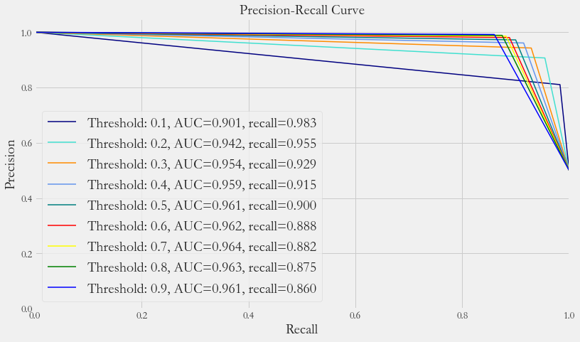
精确率与召回率
1 2 3 4 5 6 7 8 9 10 11 12 13 14 15 16 17 18 19 20 21 22 23 24 25 26 from sklearn.metrics import precision_recall_curvey_pre_proba = gs.predict_proba(x_test)[:,1 ] colors = ['navy' , 'turquoise' , 'darkorange' , 'cornflowerblue' , 'teal' , 'red' , 'yellow' , 'green' , 'blue' ] thresholds = [0.1 , 0.2 , 0.3 , 0.4 , 0.5 , 0.6 , 0.7 , 0.8 , 0.9 ] plt.figure(figsize=(12 , 7 )) j = 1 for t, color in zip (thresholds, colors): y_pre = y_pre_proba >= t j += 1 precision, recall, threshold = precision_recall_curve(y_test, y_pre) area = auc(recall, precision) cm = confusion_matrix(y_test, y_pre) r = cm[1 , 1 ] / (cm[1 , 1 ] + cm[1 , 0 ]) plt.plot(recall, precision, color=color, lw=1.5 , label=f'Threshold: {t} , AUC={area:.3 f} , recall={r:.3 f} ' ) plt.xlabel('Recall' , fontsize=20 ) plt.ylabel('Precision' , fontsize=20 ) plt.ylim([0.0 , 1.05 ]) plt.xlim([0.0 , 1.0 ]) plt.title('Precision-Recall Curve' , fontsize=20 ) plt.legend(loc="lower left" , fontsize=20 )
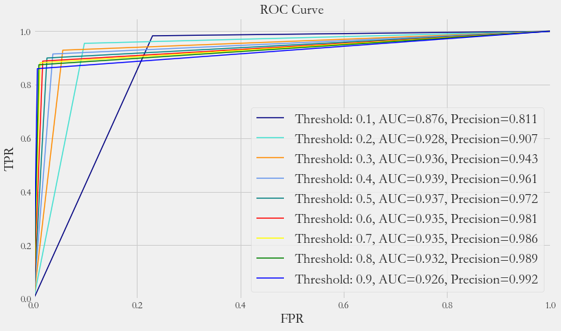
ROC曲线
1 2 3 4 5 6 7 8 9 10 11 12 13 14 15 16 17 18 19 20 21 22 23 24 25 y_pre_proba = gs.predict_proba(x_test)[:,1 ] colors = ['navy' , 'turquoise' , 'darkorange' , 'cornflowerblue' , 'teal' , 'red' , 'yellow' , 'green' , 'blue' ] thresholds = [0.1 , 0.2 , 0.3 , 0.4 , 0.5 , 0.6 , 0.7 , 0.8 , 0.9 ] plt.figure(figsize=(12 , 7 )) j = 1 for t, color in zip (thresholds, colors): y_pre = y_pre_proba >= t j += 1 fpr, tpr, threshold = roc_curve(y_test, y_pre) area = auc(fpr, tpr) cm = confusion_matrix(y_test, y_pre) p = cm[1 , 1 ] / (cm[1 , 1 ] + cm[0 , 1 ]) plt.plot(fpr, tpr, color=color, lw=1.5 , label=f'Threshold: {t} , AUC={area:.3 f} , Precision={p:.3 f} ' ) plt.xlabel('FPR' , fontsize=20 ) plt.ylabel('TPR' , fontsize=20 ) plt.ylim([0.0 , 1.05 ]) plt.xlim([0.0 , 1.0 ]) plt.title('ROC Curve' , fontsize=20 ) plt.legend(loc="lower right" , fontsize=20 )
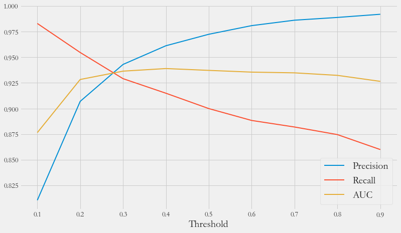
各指标走势
1 2 3 4 5 6 7 8 9 10 11 12 13 14 15 16 17 18 19 20 21 22 23 24 25 26 27 28 29 30 y_pre_proba = gs.predict_proba(x_test)[:,1 ] thresholds = [0.1 , 0.2 , 0.3 , 0.4 , 0.5 , 0.6 , 0.7 , 0.8 , 0.9 ] plt.figure(figsize=(12 , 7 )) j = 1 recalls = [] aucs = [] precisions = [] for t, color in zip (thresholds, colors): y_pre = y_pre_proba >= t j += 1 fpr, tpr, threshold = roc_curve(y_test, y_pre) cm = confusion_matrix(y_test, y_pre) area = auc(fpr, tpr) precisions.append(cm[1 , 1 ] / (cm[1 , 1 ] + cm[0 , 1 ])) recalls.append(cm[1 , 1 ] / (cm[1 , 1 ] + cm[1 , 0 ])) aucs.append(area) plt.plot(thresholds, precisions, lw=2 , label=f'Precision' ) plt.plot(thresholds, recalls, lw=2 , label=f'Recall' ) plt.plot(thresholds, aucs, lw=2 , label=f'AUC' ) plt.xlabel('Threshold' , fontsize=20 ) plt.legend(fontsize=20 )
最优阈值
Precision和Recall是一组矛盾的变量。从之前的混淆矩阵和PRC曲线、ROC曲线可以看到,阈值越小,Recall值越大,模型能找出信用卡被盗刷的数量也越多,但换来的代价是误判的数量也越大。随着阈值的提高,Recall值逐渐降低,Precision值也逐渐提高,误判的数量也随之减少。通过调整模型阈值,控制模型反信用卡欺诈的力度,若想找出更多的信用卡被盗刷就设置较小的阈值,反之,则设置较大阈值
实际业务中,阈值的选择取决于公司业务边际利润和边际成本的比较;当模型阈值设置较小的值,确实能找到更多的信用卡被盗刷的持卡人,但随着误判数量增加,不仅加大了贷后团队的工作量,也会降低误判为信用卡被盗刷客户的消费体验,从而导致客户满意度下降,如果某个模型阈值能让业务的边际利润和边际成本达到平衡时,则该模型的阈值为最优值。当然也有例外情况,发生金融危机,往往伴随着贷款违约或信用卡被盗刷的几率增大,而金融机构会更愿意不惜一切代价守住风险的底线
总结
通过信用卡欺诈预测项目,掌握了一定的机器学习技能,以及现实应用能力
而在建模过程中,特征的重要性再次体现,本次项目所提供的数据是十分规整的结构化数据,在使用逻辑回归时就能够达到93%的准确率
而在机器学习中,Precision和Recall平衡的问题,需要结合实际需求调整阈值,以达到人们所期待的效果
在现实中,银行的特征高达几千个,涵盖个人几乎所有可获得的信息,以此训练出的模型十分强大,为我们的经济安全筑起一道道高墙